
Controlling movable parts of a top-down-assembly by skeleton
Definition and transfer of the movement limits, setting the assembly constraints, creating positional representations and drawing views
Links on the topic: The Video about controlling movable parts by skeleton at Youtube or DailyMotion and the short presentation (sorry, only in German) as PDF.
How can movable parts of a skeleton-controlled assembly be controlled from the skeleton and what is this useful for?
When we design an assembly with moving parts, we need to ensure that the movement works without collisions or other problems. Without a skeleton, we would have to manually enter the relevant motion positions and conditions and manually update them with every design change. Errors often creep in. This is where skeleton modeling has another advantage: we can control the movement in accordance with the design directly from the skeleton.
In this tutorial I show a simple way to reliably and automatically control the motion states of parts in a skeleton-controlled assembly using the predominantly existing skeleton geometry. The process is:
- Create motion sketch and working geometry in the skeleton
- Create realistic constraints in the assembly with the necessary degree of freedom
- Generate end position constraints for positional representations and/or min-max conditions for real-time movement
- Generate positional representations/drawing views
Depict the movement in the skeleton part
First, the movement path must be sketched in the skeleton with all dimensionally relevant geometries, then working geometry is created as installation references for assembly.
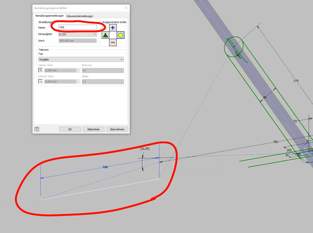
The movement path is represented by sketch(es). The defining dimensions of the movement must be present in the sketch (or multiple sketches). Controlling dimensions, reference dimensions or parameters can also be used. The dimensions or parameters should be meaningfully named (Figure 1.1) and, if necessary, marked as key parameters so that they can be easily found again later. In this case I am depicting a simple linear movement that is fully determined with a single line and a linear dimension as the stroke length.
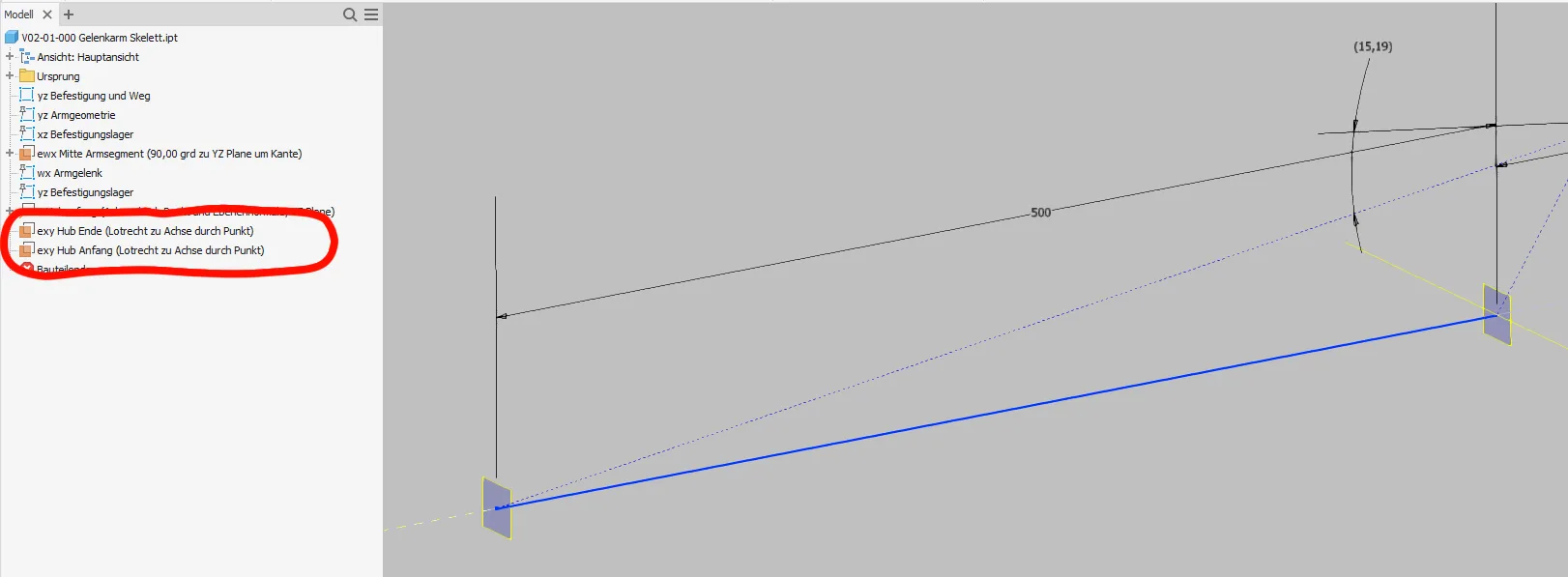
Next, the work geometry required to define the assembly constraints in the assembly is created. Planes or axes are usually the method of choice. In the example, the end of the articulated arm should move linearly, as is the case mechanically with a load guided with rollers or sliders. For such movements, two parallel planes at both ends of the stroke perpendicular to the line of movement are well suited. They can be defined stably and consistently on the end points and the line (Figure 1.2).
Creating the assembly constraints
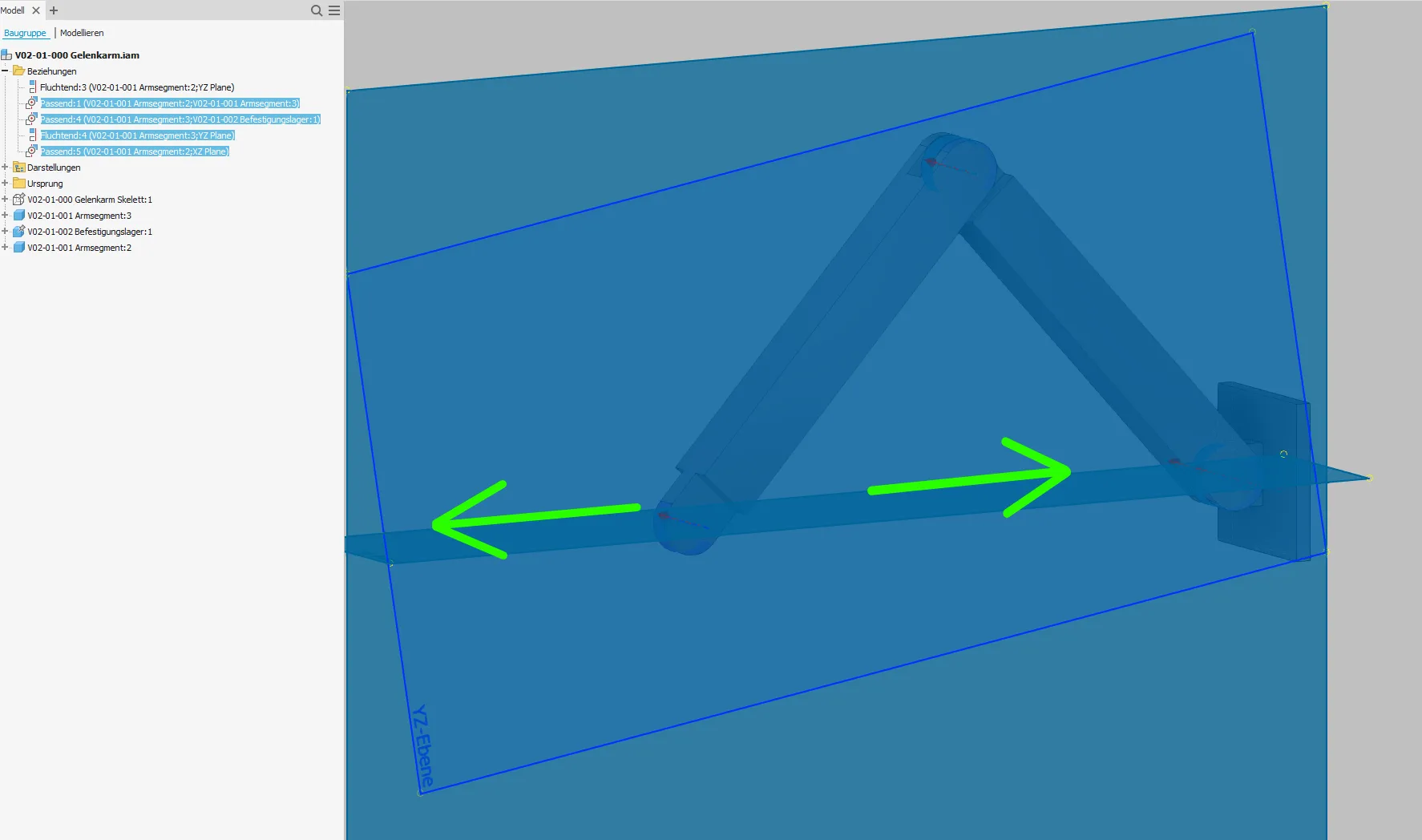
The assembly constraints of the moving parts should be as realistic as possible. If designs are still incomplete, "idealized" conditions must be created where parts will later take on this function. In this example, the arm segments are held at the midplane; This is of course unrealistic but not a problem with symmetrical assemblies. The joints that have only been hinted at so far are created as non-aligned (important!) concentric axis constraint. I assume that the end of the arm is guided linearly by parts that are still to be designed and constrain the axis at the end of the arm on the XZ plane. The end of the arm can now only move linearly in the stroke direction as shown in Figure 2.1.
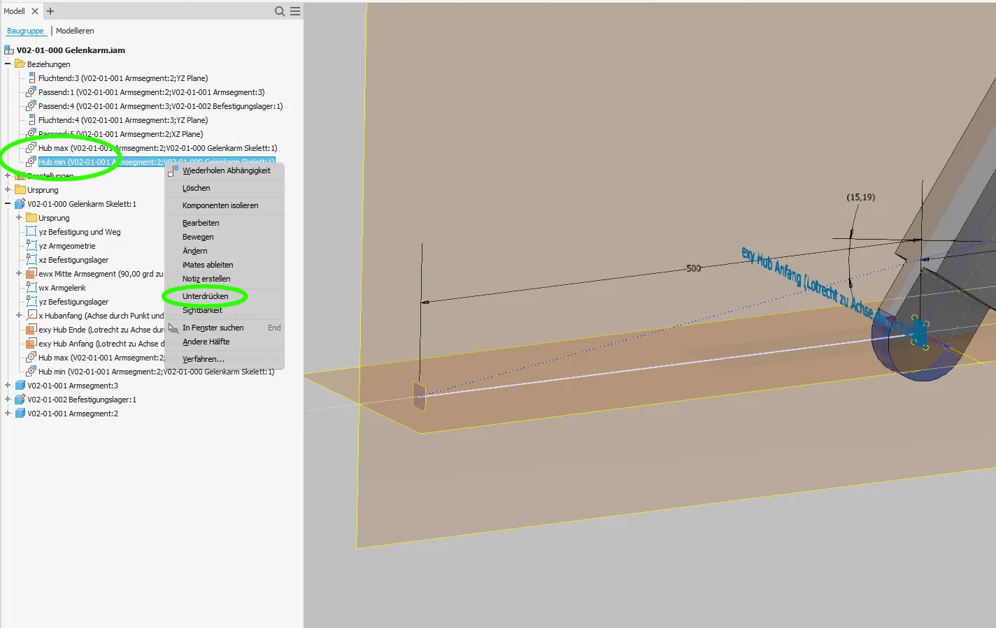
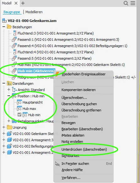
If we only want to see the end positions, we can now constrain the arm end on the work planes for the end positions of the skeleton. Accordingly, there is a condition "max stroke" and "min stroke" (Figure 2.2), which I set suppressed in the standard state as shown in Figure 2.3 and only switch them on when I want to see the respective state.
We can also use these constraints later to create positional representations.
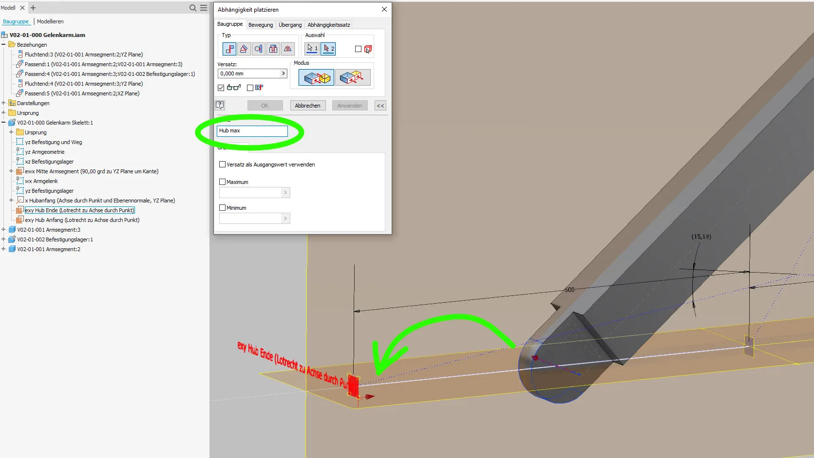
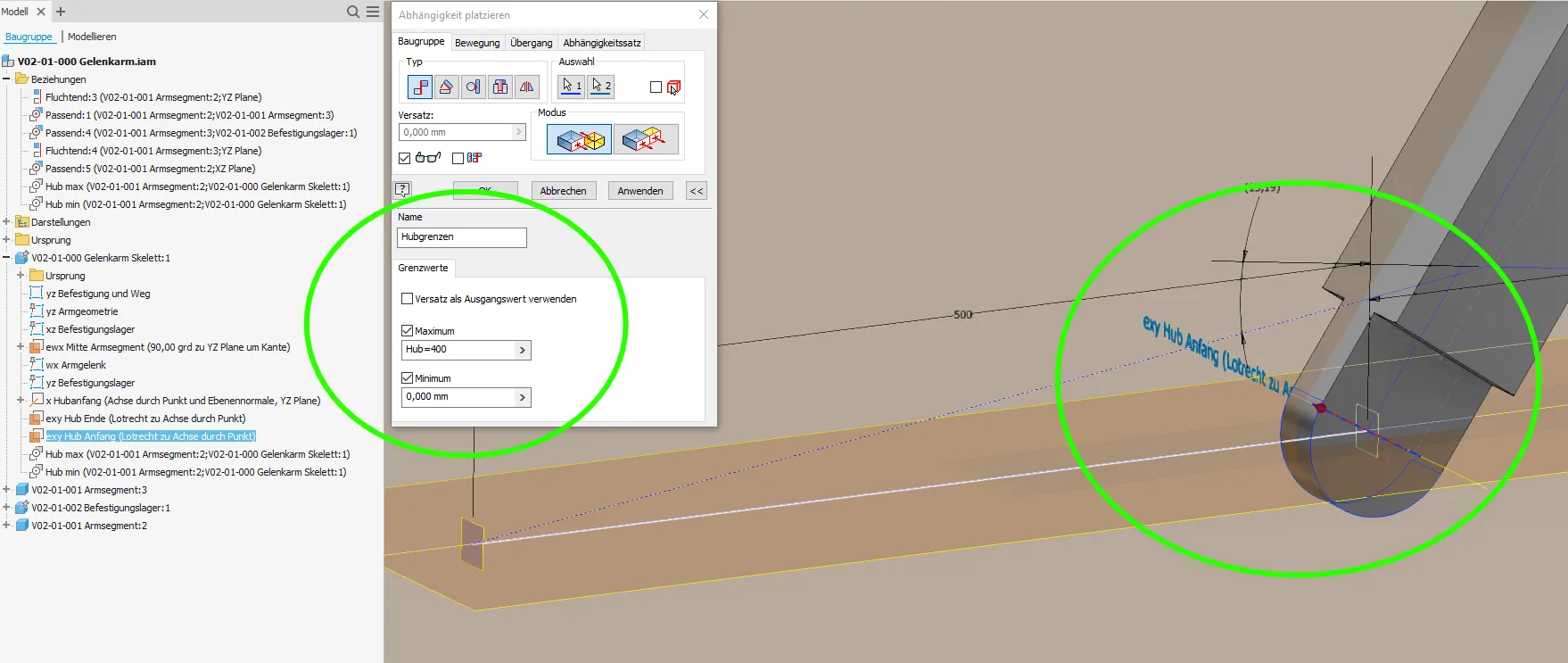
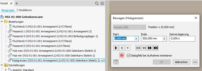
To realize realistic real-time movement with correct boundaries, we need another constraint. This means that the moving part, here the end joint of the arm, is again constrained to one of the stroke planes. The beginning of the stroke is usually a good option so that the values are positive in the direction of the functional idea. This time, however, the "limit values" fields are filled in (Figure 2.4). When filling out the maximum field, I create the variable "stroke" and initialize it with 400 mm, which does not correspond to the actual stroke in the example. So I see that the variable is not yet linked to the skeleton.
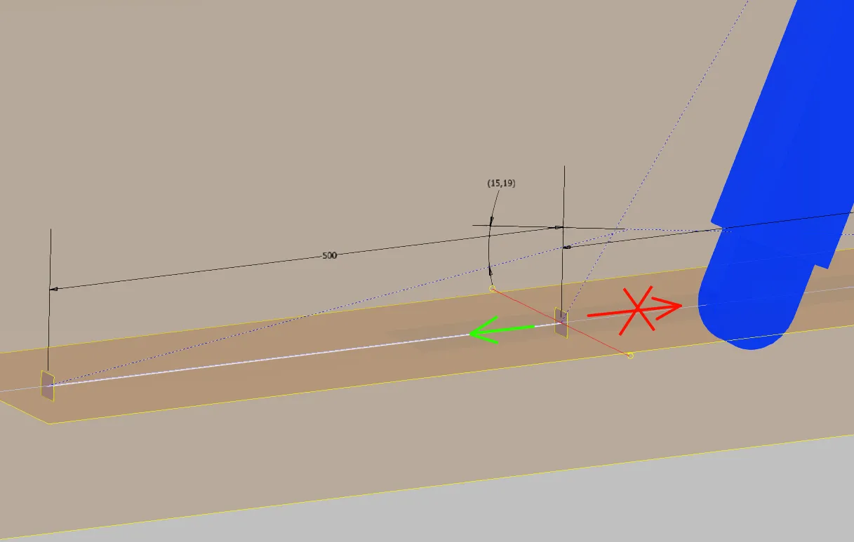
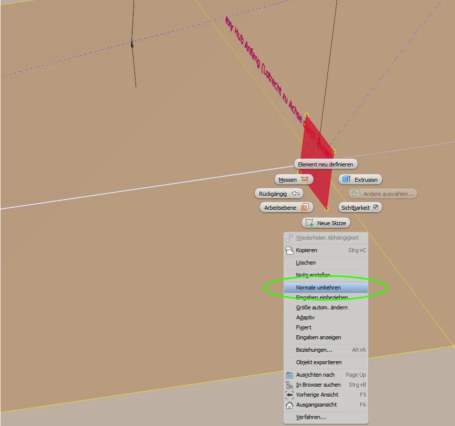
If the moving part becomes movable in the wrong direction as in Figure 2.5, the normal direction of the working plane in the skeleton can be reversed (Figure 2.6). For constraints between two surfaces, Inventor uses reference 1 to define the positive direction!
If you now drag the end of the arm with the mouse, you can drag it away from the "stroke start" plane by the set amount towards "stroke end".
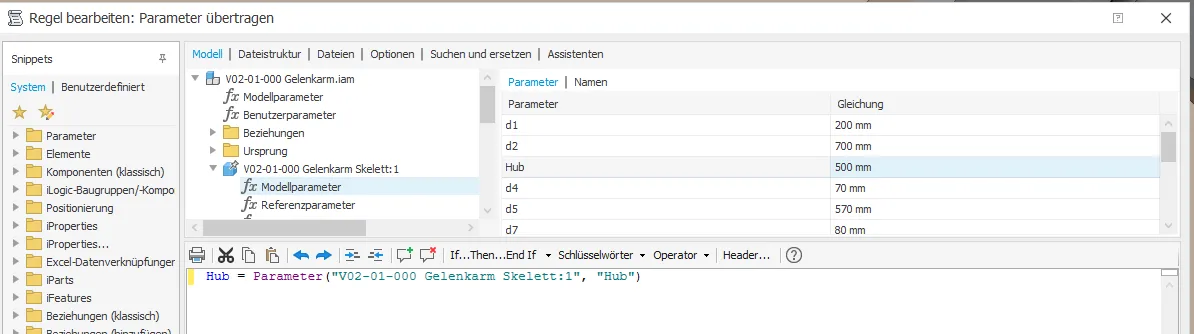
Now, to ensure that these limits always correspond to the design, we need a small iLogic rule like in Figure 2.7, with which parameters are transferred from the skeleton to the assembly. In this case, a single equation that sets the Stroke assembly parameter used in the constraint to the "stroke" skeleton dimension is sufficient. After executing this rule, the stroke maximum is set to the actual value from the skeleton. Any additional movement parameters can be added to this rule. Alternatively, you could use the Measure command in iLogic to transfer the distance between two skeletal elements into a parameter, but that seems more complicated to me.
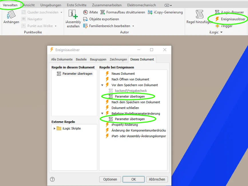
To ensure that the assembly parameters are updated automatically when changes are made to the skeleton, this rule must be executed regularly using event triggers. Depending on the required and available computing power, the variants "before opening", "before saving" or "when model parameters change" are available (Figure 2.8).
The possible stroke in the assembly and the switchable end positions now always match the stroke designed in the skeleton. This means that the automatic movement function as shown in Figure 2.9 can now also be used conveniently.
Creating positional representations and drawing views
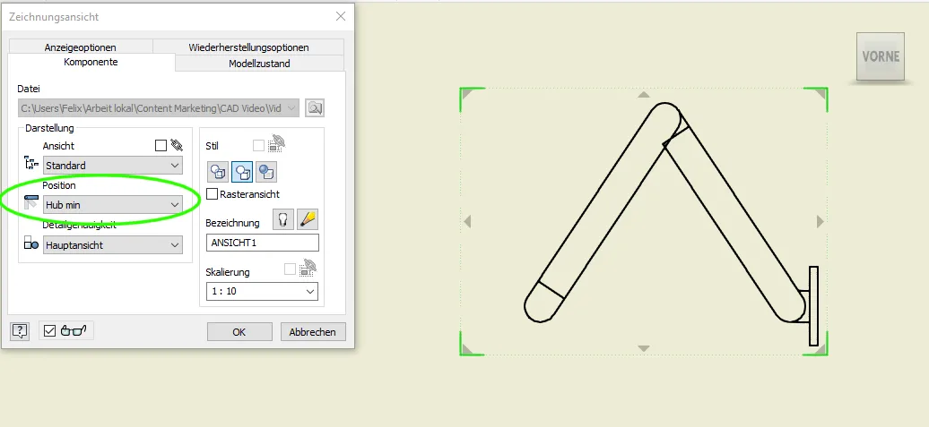
In order to be able to call up the end positions quickly or use them in drawings, a positional representation (Figure 3.1) must be created for each end position in which the corresponding end position placement condition is activated.
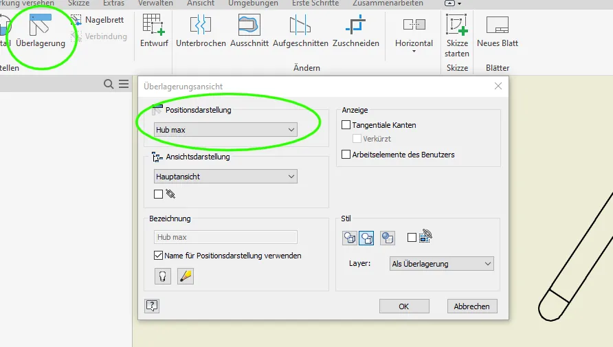
The position displays are very suitable for quickly switching through different states during presentations. They can also be used for the drawing views as shown in Figure 3.2 and to create beautiful superimposed displays such as Figures 3.3 and 3.4:
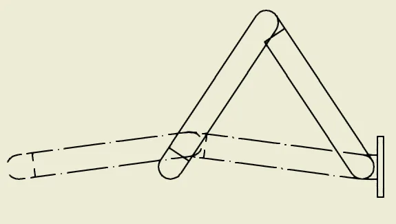
More than two positions can also be shown in one view. They all can also be dimensioned and annotated.
Closing words
The kinematics used in this example are very simple in order to explain the method in an easily digestible way. Of course, much more extensive and complex scenarios are also possible with superimposed directions of movement and intermediate states. So you still have plenty of scope for creativity!
If you need more in-depth advice on CAD methods, please click on Contact.
You are also welcome to download the short presentation (sorry, only in German) on the topic. It may be used freely in unchanged form, including commercially, provided the source is acknowledged (license: CC BY-ND).
You can also download the model files in the finished state of this tutorial.
Click the links to copy to clipboard
This page: https://r-kon.eu/cad-bewegliche-teile-mit-skelett-steuern.php
The video: https://youtu.be/MhWhVzdaSlo (Youtube) / https://dai.ly/x8peasu (DailyMotion)